NORCAL Publications

Research Article

Optimization of Large-Scale Solar Hot Water System Using Non-Traditional Optimization Technique

EB Priyanka^* and S Thangavel

Department of Mechatronics Engineering, Kongu Engineering College, Perundurai, Chennai, India

^*Corresponding author: E B Priyanka, Department of Mechatronics Engineering, Kongu Engineering College, Perundurai, Chennai, India, E-mail: priyankabhaskaran1993@gmail.com

Citation: Priyanka EB and Thangavel S (2018) Optimization of Large-Scale Solar Hot Water System Using Non-traditional Optimization Technique. J Environ Sci Allied Res 2018: 05-14. doi:https://doi.org/10.29199/2637-7063/ESAR-201017

Received: 30 April, 2018; Accepted: 14 June, 2018; Published: 21 June, 2018

Abstract

The depleting fossil fuel concerns, pollution emissions, and global warming force each and everyone towards using clean and renewable energy sources. Hot water production is one of such applications where solar energy can be used most effectively. In this project work, design, analysis, and optimization of large-scale Solar Hot Water System (SHWS) are attempted for a college hostel (having 700 students), which requires hot water for bathing purposes. The preliminary SHWS is designed based on the existing design methods. The system is modeled mathematically and a simulation program has been developed to predict thermal performance and pressure drop aspect. The preliminary calculations for determining performance characteristics and simulation methodology were carried out using MATLAB. The system performance is predicted over the life span of 10 years. Initially, the effect of collector area, storage tank volume on the performance and life-cycle cost of the system are analyzed using robust design methodology. Then the parameter is increased to four and optimization was carried out. Using the simulation, the performance of the system is analyzed for different settings. Using S/N ratio, more control parameter settings are identified so that the system is robust against the variation of noise factors. The optimum system configuration is achieved with less number of design iterations. The comparisons have been made between the optimum under four parameters using Taguchi's robust design methodology.

Keywords: MATLAB; Solar Hot Water System; S/N ratio; Taguchi’s Design Method

Introduction

Alternative energy has become important and relevant in today’s world due to the problems associated with the use of fossil fuels [1,2]. Non-Conventional Energy Sources, which comprise both renewable and nonrenewable sources, should play an increasing role in the coming periods in view of fast depleting fossil-fuel reserves and growing concerns for environmental protection. Perennial energy shortages and resulting inflation have adversely affected the balance of payment position in energy scare economies of the developing countries [3,4].

How to cost-effectively design a high-performance solar energy conversion system has long been a challenge. Solarwater heater (SWH), as a typical solar energy conversion system, has complicated heat transfer and storage properties that are not easy to be measured and predicted by conventional ways. In general, an SWH system uses solar collectors and concentrators to gather, store, and use solar radiation to heat air or water in domestic, commercial, or industrial plants [3]. For the design of high-performance SWH, the knowledge about correlations between the external settings and coefficients of thermal performance (CTP) is required. However, some of the correlations are hard to know for the following reasons: (i) measurements are time-consuming [5]; (ii) control experiments are usually difficult to perform; and (iii) there is no current physical model that can precisely connect the relationships between external settings and intrinsic properties for SWH. Currently, there are some state-of-the-art methods for the estimation of energy system properties [6,7,4] and for the optimization of performances [8-12]. However, most of them are not suitable for the solar energy system. These problems, together with the economic concerns, significantly hinder the rational design of high-performance SWH. The solar radiant flux reaches the atmosphere [11,12] is at its greatest when the earth is closest to the sun [2,6]. The areas lying between the latitudes 30° N and 30° S, which have at least 2000 hours of bright sunshine per year. The daylight hours vary from month to month. The peak insolation received on the earth’s surface is approximately 1 kW/m². The mean value of the flux reaching the outside earth’s atmosphere is called the solar constant, which is estimated as 1.353 kW/m² [6,10].

Large-Scale Solar Water System

Thermosyphon Systems [4] use a separate storage tank located above the collector. The liquid which gets heated in the collector rises naturally to the tank where it is kept until needed. A benefit of the systems is that they require no moving parts. The (Figure 1) shows a natural circulating type solar hot water system. It consists of a tilted collector, with transparent cover plates, a separate, highly insulated water storage tank, and well-insulated pipes connecting the two. The bottom of the storage tank is located at least 30cm higher than the top of the collector. Thermosiphon Systems use the natural tendency of heated water to rise and cooler water to fall to perform the heat-trapping task. The cold water pumps the water which was heated through the collector outlet and into the top of the tank, thus heating the water in the tank. The cold-water line from the accommodation location flows directly to the tank. Solar heated water flows from the tank to load whenever water is used.

 

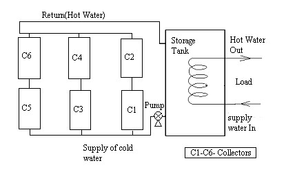
After sunset, a thermo-siphon system can reverse its flow direction and loss of heat to the environment during the night. To avoid reverse flow, a non-return valve is provided in the water inlet pipe just before the collector inlet. To provide heat during long, cloudy periods an electrical immersion heater can be used as a backup for the solar system. A non-freezing fluid should be used in the collector circuit if the atmospheric temperature falls below the freezing point of water. The thermo-siphon system is one of the least expensive solar hot-water systems and should be used whenever possible. Large arrays of flat-plate collectors are used and forced circulation is maintained with a water pump. The storage tank can be located at any convenient place as forced circulation is used. A schematic diagram of a typical closed loop system is shown in the (Figure 2). Water from a storage tank is pumped through a collector array, which performs heating and then flows again into the storage tank. The pump for maintaining the forced circulation is operated by an on-off controller, which senses the difference between the temperature of the water at the exit of the collectors and a suitable location inside the storage tank.

 

 

As the solar radiation and atmospheric air temperature vary over a day and over the year, each component needs to be mathematically modeled and assembled in an appropriate manner to simulate the total system.

Design Methodology Utilized in LS-SWHS Modeling

The performance analysis of the forced circulation solar water heating system is taken for investigation. The thermal and pressure drop behavior of the total system is investigated using a simulation approach. It has become the most familiar method for investigating the dynamic solar water heater operational behavior. MATLAB is the simulation package used throughout in order to simulate the total performance of the solar water heater system.

The problem considered to obtain hot water for bathing purpose in college hostel having 600 students.

 

Estimation of hot water requirement

No. of a student in the hostel (Ns) = 700

Mass of water per student (mass of hot water) at 45° Ws = 30 kg /day

Total mass of water required per day (Mw) = Ns^*Ws = 700^*30 = 21000 kg/day

The daily heat required (Qday) = Mw^*cp^*(tl-tfw)

Where,

Average hot water temperature required tl = 45° C (Assumed)

Supply water temperature ti = 25° C (Assumed)

Cp = 4.186 kJ/kg.K for water

Hence Qreqd = 21000^*4.186^*(45-25) = 17^*10⁵ kJ/day.

 

About 10% of students may not take bath using hot water. Hence the amount of quantity has to be reduced. However, there will losses from the system, which are about 10%, thus both mutually cancel out.

Based on the detail presented in Sukhatme (1996)

Yearly average solar radiations available on horizontal surface (Ig-day) = 5 kW hr = 5^*3600 = 18000 kJ/day

About 60% of the above quality is available on the collector surface 

ie, Rav = 0.6

Average efficiency of the collector over a day (hcol) = 35%

 Standard collector module area (ap) = 2m²

The number of collectors needed can be estimated below

Collector area required (Atot, col) = Qreqd/(Ig-day^*Rav^*hcol,day)

 = (17^*10⁵)/ (18000^*0.6^*0.35) = 450 m²

No. of collector modules needed, ncol = Atot, col/ap = 450/2 = 225

Calculation of storage tank size

Assuming the maximum storage tank temperature as Tfinal = 75(° C) (at the end of the day)

Qreqd = mwt^*cpwt^* (Tfinal-Tinitial)

i.e, 17^*10⁵ = mwt^*4.186^*(75-25)   \ mwt = 8100 kg

if Tfinal = 60° C, mwt = 11500kg.

Calculation of total mass flow rate at the collector circuit

Collector circulating pump operating hours per day = 10 (ie,7.00 am to 5.00 pm)

An average temperature rise of water across the collector is 25 (. i.e., Δtrise = 25° C.

Now,

Qreqd = 15^*10⁵ kJ/day = 17^*10⁵/(10^*3600); ie, Qcol = 47.2kW

Also,

Qcol = mtot^*cp^*Δtrise; i.e., 47.2 = mtot^*4.1186^*25;   \mtot = 0.45kg/s

Calculation of total mass flow rate in the load loop

The hot water is supplied to the hostel during 2 hours of the day 6.00am to 8.00am

Now,

Qload = 17^*10⁵ kJ/day = 17^*10⁵/(2^*3600) = 236kW

The temperature of load, Tl = 45° C (Assumed)

Supply water temperature to the tank, tsup = 25° C (assumed)

Now,

Qload = ml^*cp^*(tl-tsup); i.e, 236 = ml^*4.186^*(45-25)

                ml = 2.8 kg/s

Detail of the system after preliminary design

From the preliminary system design carried out the final details follow:

Area of each collector module (ap) = 2 m²

No. of collector modules required (ncol) = 225

Storage tank size required (volt) = 8,100 to11,500 kg

Mass flow rate in the collector circuit (mtot) = 0.5 kg/s

Mass flow rate in the collector load circuit (ml) = 2.8 kg/s

Collector pump will be operated if the total temperature rise of water across the collector circuit is 5° C. Hot water is drawn from the tank during 6.00am to 8.00am (2 hours) for each day.

Modeling of Pipeline

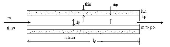
The mathematical modeling for the calculation of pipe heat loss or heat gain and pressure drop is schematically shown in (Figure 3). The pressure and the temperature decrease across the pipe and this loss are calculated using the thermal energy concepts. This pressure drop and the temperature difference are based on the physical configuration of the pipe namely the geometrical parameters of the pipe, the friction factor and also the environmental conditions on the pipe.

 

Calculation of pressure drop (Dp)

Calculating velocity of water in the pipe (V), V = (4^*m)/rp      …………(4.1)

Calculating Reynolds number (Re)

Re = (r^*V^*dp)/ m                                                                                  ………… (4.2)

If Re < 2300 Flow is Laminar

Calculating friction factor (f),

f = 64/Re                                                                                               …………. (4.3)

ElseNu = 3.66 [The values taken from HMT Data Book, Kothandaraman (1998)]

Calculating Convective resistance of inner surface (hi)

hi = (kf/dp)^*  Nu                                                                                                                            ………….  (4.4)

Else if Re > 2300 Flow is Turblent

f = [(1.82^*(log₁₀(Re)-1.62)]^-2                                                             …………. (4.5)

Prf = (cpf/kf)                                                                                        …………. (4.6)

Nu = 0.023^*(Re ^0.8)^*(prf ^0.33)                                 

hi = (kf/dp)^* Nu                                                                                   …………. (4.7)

Calculating the resistance of pipe (Rh)

Rh = (2^*f^*lp^*V)/(dp )³                                                                         …………. (4.8)

Calculating pressure drop (Dp)

Dp = Rh^*m                                                                                            …………. (4.9)

 

Calculation of fluid outlet Temperature (to)

Calculating outlet diameter of pipe

do = dp+(2^* thp)                                                                                  …………. (4.10)

din = do+(2^* thin)                                                                                …………. (4.11)

r1 = do/dp

r2 = din/do

Rwp = log(r1)/(2^*pi^*kp^*lp)                                                                 …………. (4.12)

Rwin = log(r2)/(2^*pi^*kins^*lp)                                                             …………. (4.13)

Rw = Rwp+Rwin                                                                                 …………. (4.14)

Finding inside convective resistance

Calculating inner Area of pipe (Ai)

Ai = p^*dp^*lp                                                                                         …………. (4.15)

Ri = 1/(hi^*Ai)                                                                                        …………. (4.16)

Finding outer convective resistance

Ao = p^*din^*lp                                                                                       …………. (4.17)

Ro = 1/(ho^*Ao)                                                                                    …………. (4.18)

Calculating overall loss coefficient

Rtot = Ri+Rw+Ro                                                                                …………. (4.19)

Ui = 1/(Rtot^*Ai)                                                                                   …………. (4.20)

By heat balance

Heat Loss a fluid = Heat lost by atmosphere

tm = ti (assumed)

Qloss = Ui^*Ai(tm-tsurr)                                                                      …………. (4.21)

Qfluid = m^*cpf^*(ti-to)                                                                         …………. (4.22)

The fluid outlet temperature (to)

to = ti-(Qloss/(m^*cpf))                                                                        …………. (4.23)

Modeling of Collector

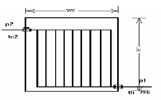
A solar collector is a special kind of heat exchanger that makes use of the high energy infra-red radiations of the solar spectrum to heat the working fluid, while conventional heat exchangers accomplish a fluid-to-fluid heat exchange with low heat content, which is a negligible factor compared to solar energy radiations. The solar collector entraps the incoming high energy solar radiations and transfers the energy to the fluid flowing through the collector in (Figure 4).

 

The radiations absorbed by flat-plate solar collectors lie in the range from infra-red to visible radiations. The radiation heat transfer is thus used in the calculation of the absorbed solar radiation and the heat gain in the solar collector. While the equations for collector performance are reduced to relatively simple forms in many practical cases of design calculations, they are presented below. Each collector is modeled using a lumped model. It requires solar radiation on the tilt surface and atmosphere temperature as inputs.

Calculation of solar radiation on the collector surface

The declination (d) is calculated as

d = 23.45 Sin [360(284+n)/365]                                                       …………. (4.24)

Local apparent time (LAT) is calculated as

Lat = time-((4^*(82.5-long)/60)+(E/60)                                             …………. (4.25)

Here, the negative sign in the first correction is applicable for Eastern Hemisphere while the positive sign is applicable for Western Hemisphere.        

Calculating hours angle (w)

w = [(12^*60)-Lat]^* (15/60)                                                                 …………. (4.26)

Calculating angle of incidence (q) for surface facing due South

q = Cos^-1[Sin d Sin (f-b) + Cosd Cosw Cos (f-b)]                       …………. (4.27)

For horizontal surface the Zenith angle (q_z) is

q_z = Cos^-1[Sin f Sin d + Cosd Cosw Cos f]                                   …………. (4.28)

Solar flux incident on collector

For beam radiation (r_b) = Cos q/Cos q_z                                                                 …………. (4.29)

For diffuse radiation

(r_d) = (1+ cosb)/2                                                                                 …………. (4.30)

For reflected radiation (r_r) = r(1-Cosb)/2                                        …………. (4.31)

Where r = Ground reflectivity = 0.2

Flux incident on top cover of the collector (I_T)

I_T = I_b r_b +I_d r_d +(I_b +I_d) r_r                                                                                                                                 …………. (4.32)

Collector Efficiency Factor

resadh = thadh/(kadh^*Do)                                                                                     …………. (4.33)

Fd = 1/((W^*Ul1)^*((1/(Ul1^*((W-Do)^*fi+Do)))+resadh+(1/(pi^*Di^*hf))));        …………. (4.34)

Collector Heat Removal Factor Ap = (L1^*W1);                                               …………. (4.35)

Fr = ((m^*cp)/(Ul1^*Ap^*3600))^*(1-exp((-Fd^*Ul1^*Ap^*3600)/(m^*cp)));             …………. (4.36)

qui = Fr^*Ap^*(S-Ul1^*(Tfi-Ta));                                                                             …………. (4.37)                                  

 

Calculating use full heat gain

 Qu = h_i^*ap^*It                                                                                                        .…………. (4.38)

Calculating collector outlet temperature C = Qu/(mflow^*cpf)                    ...…………. (4.39)

Tc2 = tfi+C                                                                                                             .…………. (4.40)

 

Calculating collector pressure drop

Calculating velocity of water in each channel of collector

Vc = (4^*mflow)/dc)²                                                                                                                 …………. (4.41)

Calculating Reynolds number (Re)

 Re = (Vc^*dc)                                                                                       …………. (4.42)

If Re <2300 Flow is Laminar

Calculating friction factor (f),

f = 64/ Re                                                                                              …………. (4.43)

Else if Re >2300 Flow is Turbulent

f = [(1.82^*(log₁₀(Re)-1.62)]^-2                                                                                            …………. (4.44)

Calculating the resistance of collector (resc)

Rc1 = (2^*f^*lc^*Vc)/(pdc)³                                                                    …………. (4.45)

IRc2 = (1/Rc1)^*ntube                                                                         …………. (4.46)

 resc = 1/IRc2                                                                                      ………….  (4.47)

Calculating collector pressure drop (Dp)

Dp = resc^*mflow                                                                                  …………. (4.48)

Modeling of storage tank

The intermittent, variable and unpredictable nature of solar radiation generally leads to a mismatch between the rate and time of collection of solar energy and the load needs of a thermal application. As a result, it is often necessary to use a storage system in between. The storage system stores energy when the collected amount is in excess of the requirement of the application and discharges energy when the collected amount is inadequate.

 

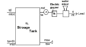
The size of a storage system is largely determined by the specific purpose for which it is used. The time interval during the day over which the energy is required is essentially the same as the time of collection. However, a storage system as shown in (Figure 5) is needed because there is some mismatch between the amount of energy required and the amount collected at any instant. The storage system in such a situation has to store energy only for short intervals of time and is relatively small in size. It is called ‘buffer storage’ the load demand shown extends overall 24 hours, whereas the collection takes place only during the sunshine hours.

Calculation of change of heat content of the storage tank

The rate of change of heat content of the tank =

{Heat added in the collector loop} - {heat removed the Load loop} - {tank heat loss}

lbyd = 2 (Assumed)

dtank = (2^*volt/pi)^(1/3)

ltank = lbyd^*dtank

ast = pi^*dtank^*ltank+(2^*pi^*dtank^*dtank)/4

Qtloss = utank^*ast^*(tt1-tsurr)

rho = 1000

mt = rho1^*volt

Q = Qcol1-Qload1-Qtloss

ttnew = (Q^*dtime/(mt^*cpt)) + tt1

 

Modeling of load loop

Calculation of load loop

Solar water heaters with larger tanks than conventional water heater tanks could have larger losses and consequently increased loads. The usual situation is to have the loads on a non-solar system equal to the loads on the solar system designed for the same task.

tsw = tsurr-5

Qreqd = mload1^*cpl^*(tload1-tsw)

if tt1 > tload1

msw = Qreqd/(cpl^*(tt1-tsw))

maux = mload1-msw

qaux = Qreqd-Qload1

Simulation Methodology

The ANOVA of each of the objective functions are considered, and the design space is reduced according to the following rules:

1. If a factor has a serious effect on all objective functions, then all the levels that optimize at least one object are selected.
2. If a factor has an important effect on a single objective, the factor level that optimizes this objective is selected regardless of its significance on other objectives.
3. If a factor has an insignificant effect on all the objectives, then the designer’s discretion is used to determine the objective most affected by this factor and the best level of the factor is identified.

Control and noise factors and their levels (for LS-SHWS)

Control factors are those, which can be controlled under normal production conditions. The control, noise and held constant parameters are identified and are presented in (Figure 6). The Robust design methodology is finding the value (system) of the control parameters in such a way that any variation in the noise parameters does not affect the output or lowest possible variation in the output. The control parameters are a number of the collector, the volume of the storage tank, mass flow through a parallel of each collector.

 

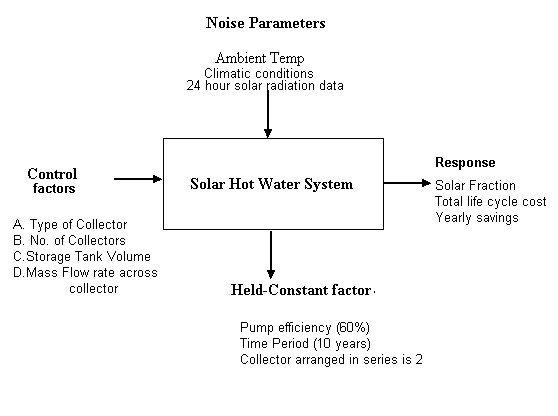
The held constant factors are the lifespan of the system is 10 (years), the pump efficiency is 60% and the arrangement of the collector in series is 2 collectors. The noise parameters are climatic conditions for winter and summer, ambient temperature and 24 hours solar radiation data. It has three level of the experiment the control parameters and two levels of noise factor (winter and summer) condition. The level of control factor is given in the (Table.1).

1. 1.  

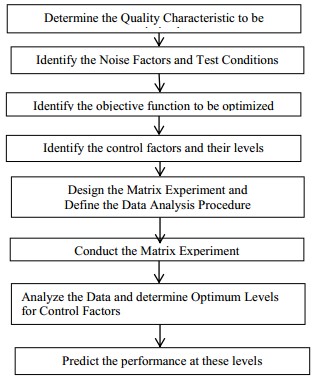
Steps in taguchi methodology: Taguchi method is a scientifically disciplined mechanism for evaluating and implementing improvements in required perspectives. These improvements are aimed at improving the desired characteristics and simultaneously reducing the number of defects by studying the key variables controlling the process and optimizing the procedures or design to yield the best results. The method can be applied to any process in engineering fabrication, computer-aided-design etc. Taguchi method is useful for 'tuning' a given process for 'best' results. Taguchi proposed a standard 8-step procedure for applying his method for optimizing any process, given in the flowchart of (Figure 7). Taguchi suggested that parameter design using noises that are deliberately created was more effective than not if noises can be created purposely. The reason is that if noise is not induced deliberately, many experiments must be performed to investigate the effects of noise factors diversely on the process and it is very difficult to obtain reliable results under different noise conditions. If the experiments can be performed under various levels of noise i.e. with positive induction of noise to the design, we can obtain a realistic level of robustness. Therefore, a characteristic of Taguchi's parameter design is the deliberate creation of noise for the identification of control factor's level that is the least sensitive to the noises. The Taguchi method, which is based on the Analysis-of-Variance (ANOVA) approach, was carried out to improve the performance of the system.

 

Orthogonal array (oa) selection and conducting experiments

To select the appropriate orthogonal array specific case study. We need to count the total degrees of freedom to find the minimum number of an experiment that must be performed to reach a near optimum parameter set. For large scale solar hot water system, the suitable orthogonal array is L9 (for control factors of 4 and 3 level) is suitable. The typical format L9 orthogonal array for experimentation pattern and results of experimentation is shown in (Table 2).

 

Result and Discussion

Determination of the optimum levels of control parameters

The traditional analysis performed with data from a designed experiment is the analysis of the mean response. The robust design method employs a signal – to –noise ratio to include the variation of response. The smallest is best type S/N ratio will be used in the analysis of the result is given in (Table 3). Since our objective is to minimize the cost we follow the smallest is best S/N ratio, which is defined as;

                         S/N = -10 log (1/n [[sigma]] y i, j²)

Since log is a monotone function, maximizing S/N is equivalent to minimizing the quality characteristic. For example for experiment 2 for the two observations under different noise conditions (n = 2) is computed as follows

S/N = – 10 log (1/2{(3.9865e⁶)²+ (7.28426e⁶)²}) = –135.36     ...… (6.1)

 

Data analysis using the S/N and ANOVA table

The analysis is made using Taguchi’s approach, which involves graphing the effects and usually identifying the factors which appear to be significant. Since the experimental design is orthogonal it is possible to separate out the effect of each factor. The average S/N ratio for each level of the four control factors are displayed in the response table given in (Table 4). The S/N ratios shown in the response table are calculated by taking the average from the Table 4 for a parameter at a given level at every time it was used. As an example, B was at level two. The average of respective S/N ratio is -135.14 which is shown in the response table under B at level 2. Analysis of variance is a computational technique that quantitatively estimates the relative contribution of each parameter variation of each parameter variation makes to the overall response variation. The ANOVA table consists of the sum of squares and percentage contribution. The sum of squares can be obtained by the formula:

Sum of Squares SS_P = (A₁²/n+A₂²/n+A₃²/n -∑y_i²/N)           ...… (6.2)

Percentage contribution P = Sum of squares of a parameter /Total sum of squares

 

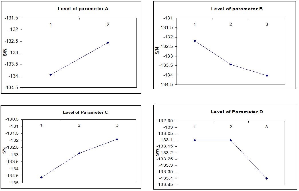
From (Table 4) the control parameter C is more significant and D has the least influence than the other parameters having the largest effect on cost. Clearly, the level 3 appears to be the best choice for A, B, and D parameter and level 1 for C parameter since it corresponds to the largest average S/N ratio. As a result of the above analysis, the near optimum levels for the four controllable parameters were selected as follows,

Test Parameters: A, B, C, D

Optimum Levels: 3, 3, 1, 3

Parameter setting (c): 100, 24000, 0.06, and (0.675, 6.6)

Using the average S/N ratios from the response table 4, the graphs are plotted for the four control parameters as shown in (Figure 8).

 

Conclusions

This research provides mathematically modeled and a simulation program has been developed using MATLAB to predict the thermal performance and pressure drop aspects. The performance of the system is predicted over the lifespan of 10 years and the effects of various control parameters on the performance of the system are analyzed. The system configuration is optimized based on the total life-cycle cost using robust design using Taguchi’s methodology. The system was basically designed for producing hot water for a hostel having about 700 occupants. The daily load period for both seasons namely summer and winter were considered based on the location and the energy required for producing hot water was calculated for both the conventional electrical heating system and solar hot water system.

Initially, four control parameters were taken and the optimization was carried out using Taguchi method. Then the percentage influences of various parameters are identified using ANOVA. Thus performing various iterations, the optimum control parameters were achieved with the objective to minimize the total life-cycle cost of the system and with a minimum pay-back period. The results obtained are more promising and seems to be practical if applied for real-time systems using solar energy concepts thus saving the depleting conventional energy sources. The optimum settings obtained are listed in the (Table 5 and 6). Therefore, in this case, optimization with four parameters resulted in a cost saving of Rs. 14,10,600 for the total span of ten years considered, which is about (32%) and a slight reduction in standard deviation.

 

 

In this paper, we have summarized our recent studies on the predictive performance of machine learning on an energy system and proposed a framework of SWH design using a MATLAB and Taguchi optimization technique. A combined computational and experimental case study on LS- SWH shows that this framework can help efficiently design LS- SWH with optimized performance without knowing the complicated knowledge of the physical relationship between the SWH settings and the target performances. We expect that this study can fill the blank of the HTS applications on optimizing energy systems and provide new insight into the design of
the high-performance energy system.

Conflict of Interest

There is no conflict of interest between the authors who are all contributed to this research work.

References

1. Hobson P A, Norton B (2013) A design nomogram for direct thermosyphon solar-energy water heaters. Sol energ 43: 85-95.
2. Lu S M, Li M, Tang J C (2015) Optimum design of natural circulation solar-water-heater-by the taguchi method. Energ 28: 741-750.
3. Adnan Shariah, Bassam Shalabi (1997) Optimal design for a thermosyphon solar water heater. Renew Energ 351-361.
4. Duffie J A, Beckman W A (2009) Solar energy of thermal processes.
5. Arkar C, Medved S, Novak Patik (2016) Long-term operation experiences with large-scale solar systems in slovenia. Renew Energ 16: 669-672.
6. Bryne D, Taguchi S (2010) The Taguchi Approach to Parameter Design. ASQC Quality Congress Transaction 34: 165-168.
7. Buckles W E, Klein S (2011) Analysis of solar domestic hot water heaters. Sol energ 25: 417-124.
8. Fisch M N, Guigas M, Dalenback J O (2014) A review of large-scale solar heating systems in europe. Sol Energ 63: 355-366.
9. Goyal A K, Ashvini Kumar, Sodha M S (2012) Optimization of a hybrid solar forced-convection water heating system. Energy Convers Mgmt 27: 367-377.
10. Habali S M, Hamdan M A S, Jubran B A, Adnan I O Zaid (2014) Optimization of Insulation Thickness in a Long Term Solar Storage System. Sol Wind Tech 5: 75-82.
11. Hariprasad Reddy K, Ramamoorthy B and Kesavan Nair P (2015) Application of Taguchi techniques to determine optimum grinding conditions. Renewable energy 45: 879-884.
12. Krause M, Vajen K , Wiese F, Ackermann H (2016) Investigations on Optimizing Large Solar Thermal Systems. Sol Energ 73: 217-225.