Research Article

Applying Task Scheduling for Iomt-Cloud Business Optimisation Using AI

Adedoyin A. Hussain1*, Fadi Al-Turjman2

1Computer Engineering Dept. and Research Centre for AI and IoT, Near East University, Nicosia, Turkey
2Intelligence Engineering Dept. and Research Centre for AI and IoT, Near East University, Nicosia, Turkey

*Corresponding author: Dr. Adedoyin A. Hussain, Computer Engineering Dept. and Research Centre for AI and IoT, Near East University, Nicosia, Mersin 10, Turkey. Telephone No: +905338226876; Email:hussaindoyin@gmail.com
Received Date: 12 January, 2021; Accepted Date: 11 March, 2022, Published Date: 18 March, 2022

Abstract

The IoMT-cloud enables a surplus extent of customers to get disseminated, versatile, and virtualized gear just as programming structure over the Internet. The IoMT-cloud is one of the principal headway used recently, it grants customers to get cloud resources over the internet remotely. Hence, we need to complete a reasonable task scheduling estimation to tolerably and viably meet these requests. The scheduling of task issue is perhaps the most essential issue in the IoMT-cloud since cloud execution depends prevalently upon it. Capable task scheduling administration should meet customer’s requirements and improve the resources used to overhaul the introduction of the IoMT-cloud framework. To deal with this issue, in this investigation, we attempt to show the two most notable static and one dynamic task scheduling execution separately, short job first (SJF), first come first serve (FCFS), and round-robin (RR). Likewise, it was advanced using the AI technique known as genetic algorithm (GA). The CloudSim simulation framework is used to measure their impact on total execution time (TET), algorithm complexity, throughput, resource utilization, total waiting time (TWT), availability of assets, total finish time (TFT), cost, and resource utilization. The model proposed is to improve the viability of task scheduling for the IoMTcloud stage with the best execution rate of 32.47ms. The exploratory results show that GA cuts down the cost of planning and reduces the total time, which is a convincing computation for the IoMT- cloud task scheduling.

Keywords: Cloud; IoMT; Artificial Intelligence; Shortest Job First; Round Robin; Genetic Algorithm; First Come First Serve.

Introduction

The IoMT-cloud is advanced with the improvement of PC and organization innovation. This is a result of joining circulated innovation, equal processing, and virtual innovation. A suitable scheduling methodology is utilized to assign the subtasks to the hubs of the asset center. The essential guideline of IoMT-cloud is that the framework partitions jobs presented by clients into a few free subtasks. Hence, task scheduling in a cloud environment is one of the critical advances of IoMT-cloud computing, which influences the entire execution of the computing stage. When the preparation of all subtasks is finished, it brings about asset hubs which are given back to clients by the technique [1,2]. Authors in [3] presented a task scheduling calculation in the cloud for addressing the cloud task scheduling dependent on improved scheduling calculation, which can acquire more modest time and lower cost for finishing the task. An enormous number of studies show that the issue of IoMTcloud scheduling is identified with NP-hard problem, which has been concentrated by numerous researchers. While authors in [4] receive the particle swarm optimization (PSO) to consider the nature of administration of clients, which has accomplished great outcomes in the field of planning of assets of cloud task in completing an enormous number of logical registrations. Authors in [5] proposed a genetic simulated annealing calculation for task planning with
double fitness, which can successfully adjust the requests of the clients for the properties of assignments and improve the clients’ fulfillment in the distributed computing stage. Authors in [6] utilize the system of addressing the cloud task scheduling by unique self-adjusting subterranean ant colony calculation (ACO), which beats the lack of subterranean insect province calculation in tackling the IoMT-cloud task scheduling. It includes the moderate pace of assembly and is simply trapped in a local optimum. In any case, because of the heterogeneity of the IoMT- cloud stage, any single calculation is anything but difficult to fall into local optimum, and the improvement of the calculation is centered around the idea of the calculation itself, overlooking the job of the development of information during the time spent Ä±n processÄ±ng.

To improve the effectiveness of task scheduling for the IoMT-cloud stage, a task scheduling technique dependent on hereditary calculation is introduced. Task calculation is a sort of clever advancement dependent on the twofold layer development system of information, which acquires valuable information and data through the advancement space of miniature level and saves it in the development space of large scale level, and uses those information to control the transformative cycle of principle population space [7-11]. The scheduling in IoMT- cloud is are outlined in figure 1 beneath. It is the principal innovation that utilizes the idea of business execution of software engineering with public clients [12]. IoMT-cloud is another innovation gotten from lattice processing and conveyed figuring and alludes to utilizing registering assets as an administration and give to recipients on interest through the Internet [13]. It depends on dividing assets between clients using the virtualization procedure. In any case, there are numerous difficulties common in IoMT-cloud computing, High execution can be given by computing, to get less holding up time, execution time, most extreme throughput, and abuse of assets viably. Task scheduling and load balance are the main factors in scheduling that it is viewed as the fundamental factors that control other execution models, for example, accessibility, versatility, and power utilization.

Task scheduling is one of the central issues in IoMTcloud computing. The significant favorable position of in IoMT-cloud task scheduling.

Figure 1: Illustration of the IoMT-cloud platform. This illustration shows how IoMT devices are connected to the cloud. This depiction shows the working principle of the IoMT-cloud stage. In the diagram the IoMT devices connect to the cloud via WiFi or cellular connection, afterwards, the cloud device management manages the devices on the cloud following its task scheduling criteria.

Figure 1: Illustration of the IoMT-cloud platform. This illustration shows how IoMT devices are connected to the cloud. This depiction shows the working principle of the IoMT-cloud stage. In the diagram the IoMT devices connect to the cloud via WiFi or cellular connection, afterwards, the cloud device management manages the devices on the cloud following its task scheduling criteria.

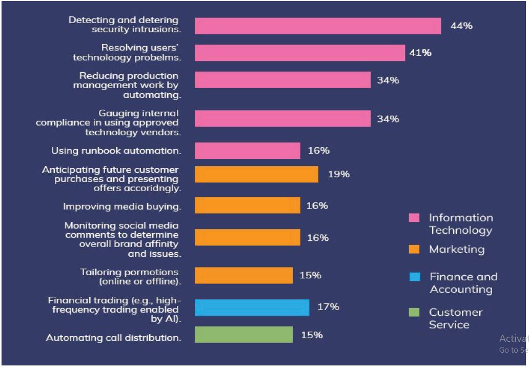
Figure 2: Illustration of the IoMT-cloud Trends [17]. This depiction shows the growing trends on the IoMT-cloud stage. The highest market growth is in
detecting and deterring security intrusions.

• Sorted the various techniques for task scheduling for IoMT-cloud.

• A depiction and description of the outcome gotten from the experiment.

• A summation of key issues and difficulties in this paper.

The paper is introduced as follows. The introduction of comparable investigations which adds to the idea of the examination and the assessment of the systems and methods utilized are introduced in section 2. While in section 3 depicts the strategy just as the materials utilized in experimenting. In section 4, sets forth the outcome and results gotten from the experiment. At long last, section 5 presents the end and conclusion of the commitments introduced in this paper. Table 1 gives an outline of the abbreviation utilized and its definition.

Literature Review

Numerous specialists have proposed answers to defeat the issue of scheduling and asset designation. This segment gives a concise survey of scheduling planning and asset allotment. Notwithstanding, further enhancements can even now be made. This current strategy gives an expense and time model for distributed computing. Authors in

[17,18] proposed a multi-object approach that utilizes the improved differential calculation. In any case, varieties in the errands are not considered in this methodology. The creators
considered the invigorate seasons of the worker in satisfying solicitations. Authors in [19] proposed a heap adjusting and planning calculation that doesn’t consider work sizes. This
approach doesn’t show the legitimate use of assets. Authors in [20] presented the planning of assignments dependent on an excursion lining model. A nonlinear programming model
has been shaped to distribute assets to errands. However, authors in [21] proposed the scheduling of errands while thinking about data transmission as an asset. Creators have
outlined the connection between task scheduling and energy protection by asset allotment. Authors in [22] proposed AHP positioning-based undertaking planning. Authors in

[23] acquainted Real-time tasks-oriented energy-aware scheduling design which plans continuous undertakings. The proposed framework doesn’t zero in on prematurely ending
resource positions and starvation. Thus, authors in [24] proposed planning for equal outstanding burdens. Creators have utilized the FCFS to deal with request occupations when assets are accessible. Multi measures choices and numerous credits are thought of. Authors in

[25] proposed a need-based employment scheduling calculation for use in distributed computing. Authors in [26] proposed the utilization of meta-heuristic improvement and particle swarm streamlining to lessen execution costs through planning. In [27] they presented the advanced expense of energy and minimise its consumption. However, in [28] they proposed the utilization of altered

Terms	Meaning
ICT	Information and Communication Technologies
SJF	Shortest Job First
SaaS	Software as a Service
IaaS	Infrastructure as a Service
RR	Round Robin
ML	Machine Learning
AI	Artificial Intelligence
GA	Genetic Algorithm
NP	Nondeterministic Polynomial
IoMT	Internet of Medical Things
ACO	Ant Colony Optimisation
TWT	Total Waiting Time
TFT	Total Finish Time
PSO	Particle Swarm Optimization
TET	Total Execution Time
QoS	Quality of Service
PaaS	Platform as a Service
PC	Personal Computer

Table 1: List of abbreviations.

insect province enhancement in burden adjusting. This framework doesn’t think about the accessibility of assets or the heaviness of errands. This technique improves the makespan. Authors in [29] proposed a framework dependent on a multi-standards calculation for planning worker load. Authors in [30] proposed an asset designation issue that means to limit the all-out energy cost of distributed computing frameworks while meeting the predetermined customer level SLAs from a probabilistic perspective [31- 33]. Thus, in [34] they proposed a framework dependent on the need for performing separable burden scheduling that utilizes logical progression measures. Here, creators have applied an opposite methodology that applies a recourse if the customer doesn’t meet the SLA arrangements. While in [35] they presented an analysis of load balancing in cloud conditions. This model robotizes the scheduling cycle and lessens the part of human directors. A few creators have executed a heuristic calculation to tackle task planning and asset assignment issue depicted previously. Likewise, in [36] and [37] they centered on planning undertakings using tree networks technique while thinking about different imperatives. This cutting edge persuades the creators of
this examination to direct extra research on assignment scheduling and asset designation.

Authors in [38] proposed a viable burden adjusting calculation by utilizing hybridization of insect province improvement method, insect settlement min-max procedure, and hereditary calculation. The movement is finished utilizing Ant Colony Optimization (ACO) scheduling calculation. They built up this powerful procedure to limit the expense of relocation of VM and keep up the SLA (Service Level Agreement) which is a QoS factor. This, at last, computes the quantity of cycle of virtual machines from its applications. As GA haphazardly chooses the processors and afterward applies the hereditary calculation, the fittest processors find the opportunity, and the VM which has lower need starves. Authors in [39] thought of the strategy that manages thestarvation issue in job adjustment. Through this, the need is allocated to VM to expand the reaction of the framework and to accomplish better burden adjusting. To conquer this difficulty they utilized hereditary calculation with the logarithmic least square method. This technique recognizes the sound chromosome, bunches the assets, applies a competition determination, and creates a new population. With this, authors in [40] have proposed an Improved GA by utilizing the processor power resource management (PPRM). Consequently, it assists with expanding the reaction time which prompts better execution of the framework and looks after consistency. After this cycle, GA is applied to the new population and finds wellness esteem. Choice, hybrid, and transformation with the flipping of parallel pieces are done. Authors in [41] have reviewed insightful cloud calculations
to adjust the heap and proposed AntLion Optimizer (ALO) to give better outcomes in adjusting the heap in the cloud.
This gives more significant arrangements. ALO handles huge issue space.

Authors in [42] have reviewed transformative GA for creating an answer. It is following three main activities. Essential GA having terms called population, chromosome, and fitness. By this thought, they accomplished bettern normal reaction time and increments cloudlets with change encoding. They have considered a need-based introductory assessment. Authors in [43] have proposed a Cloud-based general Storage and dynamic Multimedia Load Balancing (CSdynMLB) strategy to adjust the task grouping. It assists with lessening overhead, moving time and improves the exhibition. In an interactive media framework, when a customer demands a worker utilizing asset director, extra RAM limit, CPU, and extra room is needed for correspondence between the customer and the grouped worker. They have presented Job Unit Vector (JUV) and Processing Unit Vector (PUV) terms to get the fitness. Authors in [44] have proposed cross breed hereditary calculation and gravitational copying nearby inquiry (GA-GEL) calculation for VM load balance in the cloud. The comparative need is applied to all the solicitations and guarantees better QoS, high interoperability,and versatility. The result appeared with Cloud Analyst reproduction device that varies with a various number of server farms. Authors in [45] have proposed Genetic Ant Colony Algorithm-Virtual Machine Placement (GACA-VMP) way to deal with resolving VMP issues utilizing improved ACA. Through this methodology, they have chosen a doable way in two stages. This is acquired to effectively choose the actual worker and build the presentation [46-51].

Methodology

This is the systems method, design, and architecture. This is a conventional depiction and it depicts the proposed system overall. This section incorporates the direct design and more perspectives on the framework that will work inseparable while using the general framework and it is portrayed in figure 3. Besides, it also depicts the planning of the structure which incorporates portions of the system and the improvement of the structure.

Description of the IoMT-cloud scheduling model

The fundamental highlights of IoMT-cloud are selfoverhauled, per-utilization metering and charging, flexibility, and customization. The IoMT-Cloud has various qualities which offer advantages to the end client, idealistic highlights of cloud assets are basic to allow administrations that certainly establish the Cloud display and fulfill assumptions for buyers. The framework plans to improve the exhibition of task planning, while at the same time decreasing computational expenses. For these highlights, the executives assume a significant job. A key target is to anticipate the ideal calculation for approaching information when required. Additionally, we break down the prerequisites and results of using Quality of Service (QoS) with the proposed result. To accomplish this, we play out a methodical examination of static and dynamic scheduling for the IoMT-cloud as the baselines. The scheduling calculation should be adequately competent to deal with the issues identified with the task scheduling like asset dispute, shortage of assets, overprovisioning of assets, and asset fracture.

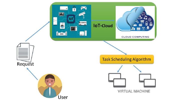
Figure 3: The proposed system architecture. This architecture shows the abstract on how our system will operate. The user sends a request for the job he wants.
The IoT-cloud platform responds to this request based on the best task scheduling algorithm and then answers the request using a virtual machine to the user.
The whole process shows the abstract of task scheduling on the IoT-cloud stage.

For the methods of scheduling IoMT-cloud assets, the cycle of Task Scheduling teaches the scheduler to get errands from the clients and request the cloud information service (CIS) for accessible assets and their properties. The clients demand the assets on interest, and the cloud supplier is responsible for the allotment of expected assets to the client to maintain a strategic distance from the infringement of the Service Level Agreement (SLA). Cloud scheduler is capable to plan various virtual machines (VMs) to various undertakings. The task scheduling framework in the IoMTcloud is portrayed in figure 4. The planned scheduling structure is made in three segments, static scheduling, dynamic scheduling, and the use of AI. While in figure 5 it shows the primary cycle of scheduling which is in three phases. The static scheduling area will utilize two notable calculations (SJF and FCFS). The dynamic scheduling area will utilize the round-robin (RR) scheduling method. The AI area will utilize a genetic algorithm (GA) and the portrayed result provides the outcome by distinguishing the one with the best outcome. It analyses them based on different related boundaries and discovers the benefits and negative marks of these calculations. This is zeroing in on the different scheduling algorithms for IoMT-cloud environment.

The static task scheduling section can be subdivided into:

• First come first serve (FCFS)

• Shortest job first (SJF)..

The dynamic task scheduling section can be subdivided into:

• Round robin (RR).

AI section is subclassed into:

• Genetic algorithm (GA).

Static task scheduling

In static scheduling, the task assigned to processors is assigned before program execution starts. An undertaking is constantly executed on the processor to which it is allocated;

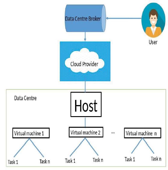
Figure 4: The task scheduling architecture. This shows the working principle on the IoT-cloud stage. The data center broker is between the user and the cloud provider. The data center broker checks for available resources and the resources present. This information is stored in a depository. The data centre contains various hosts and equipment based on the hardware property. Each host might have multiple virtual machines. Once a data centre is created it is stored in a cloud information service with the data centre broker. When a user makes a request it is sent to the data centre broker, the data centre broker checks for resource availability and responds to the request based on the scheduling algorithm, and then finally to the virtual machine for the users.

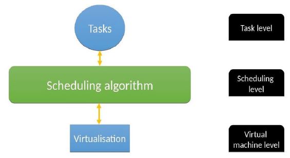
Figure 5: Task scheduling system phase. The task scheduling is divided into three phases or levels. The first level is the task level where users request a particular task. The second phase is the scheduling level where the best scheduling algorithm is applied and finally the virtual machine level which is a set of policies to distribute tasks to the virtual machine.

that is, static scheduling techniques are nonpreemptive. Considering this objective, static scheduling strategies endeavor to foresee the program execution at the accumulated time, that is, gauge the cycle or undertaking, execution times, and correspondence delays, play out a parceling of smaller errands into coarser-grain measures trying to lessen the correspondence costs and assign cycles to processors. Normally, the objective of static scheduling techniques is to limit the general execution time of a simultaneous program while limiting the correspondence delays. Moreover, static scheduling experiences numerous drawbacks. The significant favorable position of static scheduling techniques is that all the overhead of the planning cycle is caused at assemble time, bringing about a more productive execution time contrasted with dynamic scheduling strategies. Maybe perhaps the most basic deficiencies of static scheduling are that creating ideal timetables is an NP-hard issue. The utilized static scheduling method is described below.

Application of first come first serve (FCFS) in IoMTcloud: In this calculation, requests that shows up first are served first. Occupations new to the line are embedded into the tail of the line. In this model, the request for errands in the undertaking list depends on their arrival at that point doled out to VMs. This is one of the mainstream scheduling calculations and it is more attractive than other scheduling calculations. Individually each cycle is taken from the head of the line. This calculation is direct and speedy. It relies upon the FIFO rule in planning tasks with less intricacy than other scheduling calculations. It doesn’t give any need to errands. To quantify the exhibition accomplished by this strategy, we will test them and afterward estimate their effect on TET, TWT, and TFT because the errands have high holding time. Its execution with assets is not burned-through in an ideal way. That implies when we have huge requests at the start of the assignments list, all errands should stand by for a while until the huge request are through. The FCFS will have these valuable attributes:

• This sort of calculation doesn’t function admirably with delaying delicate traffic as waiting time and deferral are generally on the higher side.

• There is no prioritization at all and this makes each cycle at the end finish before some other cycle is added.

• As setting switches possibly happens when a cycle is ended, in this way no cycle organization is required and there is little planning overhead.

The handling in this approach happens by picking the correct request of tasks from the arrival. The datacentre regulator looks for a virtual machine that is free or overburden. The assignment of solicitation happens in two different ways. At that point, the main solicitation from the tasks is taken out and is passed to one of the VM through the VM scheduler. Initially, the solicitations can be orchestrated in a way and also by allotting weighty burden-less work and low burden work. The entire instrument of the calculation is portrayed in figure 6. Many functional boundaries can be considered in calculating the complex load weighing variable and current load weighing variable for each task.

Application of shortest job first (SJF) in IoMT-cloud: Need is given to assignments dependent on the length of the task and starts from the least to the most noteworthy need. In this model, errands are arranged dependent on their need. The cycle is then allotted to the processor that has the smallest bust time. The calculation is a pre-emptive that chooses the waiting cycle that has the least execution time. It has an average minimum waiting time among all scheduling calculations. The stand-by time is normally lower

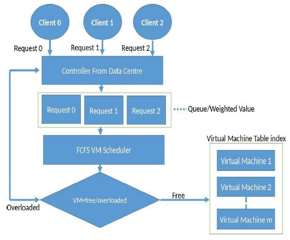
Figure 6: First come first serve scheduling algorithm. This shows the flow chart of the working principles of the first come first serve. The user or the client sends a request. The request is arranged sequentially. The first request is responded to regardless of the time. Once the first come first serve algorithm is applied, it checks for the availability of the possible resource and is then executed using a virtual machine.

Figure 7: Shortest job first scheduling algorithm. This shows the flow chart of the working principles of the shortest job first. The user or the client sends a request. The request is arranged in an orderly manner. Once the shortest job first algorithm is applied the jobs will be arranged in orderly with the shortest job first before considering the longer ones. Once the shortest job first algorithm is applied, it checks for the availability of the possible resource and is then executed using a virtual machine.

than FCFS. It possesses an injustice to certain jobs when jobs are allotted to VM. This is because of the long jobs tending to be left holding up in the assignment list while little jobs
are allocated to VM. However, it has a long execution time and TFT. The flowchart of the execution cycle is portrayed in figure 7. It will have these worthwhile attributes:

• It diminishes the normal waiting time as it executes little cycles before the execution of enormous ones.

• One of the issues that SJF calculation is that it needs to become more acquainted with the next processor demand.

• When a framework is occupied with countless minima cycles, starvation will happen.

Dynamic task scheduling

This model is implemented by moving assignments from the vigorously stacked processors to the softly stacked processors called load offsetting with the point of improving the presentation of the application. Dynamic scheduling depends on the reallocation of cycles among the processors during execution time. All things considered, all processors send their heap data to a focal processor and get load data from that processor. Many joined strategies may likewise exist. For instance, the data strategy might be incorporated yet the exchange and position approaches might be conveyed. This agreeable approach is frequently accomplished by an angle appropriation of burden data among each component. The adaptability inalienable in unique task scheduling considers variation to the unanticipated requests at run-time. The benefit of dynamic scheduling over static scheduling is that the framework does need not to know about the run-time conduct of the applications before execution.

Application of round Robin (RR) in IoMT-cloud

In this model new cycle is added to the back of the prepared line and afterward, new cycles are embedded in the tail of the line. On the off chance that the cycle isn’t finished before the lapse on processor time, at that point the processor takes the following cycle in the holding state in the line. In this kind of calculation, measures are executed at the same time as in FIFO, however, they are confined to processor time known as time-cut or quantum time. It will have these favorable attributes:

• If we apply any quantum time, at that point it will bring about a poor reaction time.

• If we apply a more limited time-cut or quantum, at that point all things considered there will be a lower CPU productivity.

The proposed scheduling count depends on actualizing the cooperative scheduling estimation. Instead of giving static TET in the CPU scheduling, our calculation calculates the TET itself. It lessens the WT and TFT profoundly appeared differently about other scheduling. Fundamentally, this is an examination proposal where the RR scheduling is contrasted to the static type. By then in the ensuing stage, the calculation calculates the TFT of the significant number of systems. At first, we will keep all the strategies in the subjective solicitation as they show up. In the last stage, the calculation chooses the first methodology from the line and distributes the CPU for a period interval of the mean TET. In the wake of determining the mean, it will characterize the TFT capably. The flowchart is portrayed in figure 8.

Application of AI

Artificial intelligence application in the IoMT-cloud is the converging of AI abilities of man-made brainpower with cloud-based conditions, making natural, associated encounters conceivable. Gigantic strides in AI, alongside a setup cloud environment, are making way for more effectiveness, adaptability, and key understanding than the world has seen so far. Computerized colleague administrations join a consistent progression of man-made consciousness innovation and cloud-based registering assets to empower clients to hinder purchases, to change a smart indoor regulator, or hear the main tune immediately. This will permit frameworks to run routine tasks altogether all alone, giving IT groups more opportunity to zero in on essential capacities, which offer more benefit, add to more creadily administration, and lift the main concern. These preferences give scheduling improvement productively. Computer-based intelligence will likewise assume a part in computerizing center cycles. We can produce AI models when a huge arrangement of information is applied to
specific calculations, and it gets essential to use the cloud for this. As we give more information to this model, the expectation improves and the precision is improved. The models can gain from the various examples which are gathered from the accessible information. For example, for ML models which distinguish tumors, a large number of radiology reports are utilized to prepare the framework. The information is the necessary info and this comes in various structures of crude information, unstructured information, and so on. This example can be utilized by any industry since it tends to be redone dependent on the venture’s needs. On account of the high-level calculation strategies which require a mix of CPUs and GPUs, cloud suppliers presently furnish virtual machines with amazingly groundbreaking GPUs. IaaS additionally helps in taking care of prescient examination. A representation of AI in assignment scheduling is portrayed in figure 9. Likewise, AI errands are currently being computerized utilizing administrations that incorporate cluster preparing, serverless processing, and coordination of holders.

Application of Genetic Algorithm (GA) for optimization in IoMT-cloud: In GA, every chromosome is a potential answer for an issue and is made out of a series of qualities. GA depicts a population enhancement strategy based on a representation of the advancement cycle of nature. The underlying population is taken arbitrarily to fill in as the beginning stage for the calculation. To get an effective GA we will apply dynamic round robin on it to form HGA. Based on fitness variables gotten from the application of the dynamic round robin, chromosomes are chosen and mutation and crossover are performed on them for the new population. A fitness variable is characterized to check the reasonableness of the chromosome for the population. The fitness variable assesses the nature of every posterity. The GA and HGA will be used interchangeably. The genetic algorithm optimization scheduling calculation is depicted in figure 10. The cycle is rehashed until adequate posterity

Figure 8: Round robin scheduling algorithm. This shows the flow chart of the working principles of the round-robin. The user or the client sends a request. The request is arranged in an orderly manner like the first come first serve. Then the CPU allocation process starts. A quantum time is given to all requests for task fairness. All request uses the same time
regardless of the order of job or time. Once the round-robin algorithm is applied, it checks for the availability of the possible resource and is then executed using a virtual machine.

Figure 9: AI application in IoMT-cloud optimization scheduling System.This shows the abstract flow chart of the working principles of the proposed AI model. The user or the client sends a request then the proposed AI model is applied to it and finally, it will be virtualized using the available virtual machine.

is made. The flowchart of GA in the IoMT-cloud is depicted in figure 11. The HGA calculation for optimization of the scheduling issue in IoMT-cloud is demonstrated as follows:

• Initialization: Generate introductory population P comprising of chromosomes.

• Perform round robin and Fitness calculation: The dynamic round robin will be performed on each chromosome process and afterwards calculate the fitness estimation of every chromosome utilizing fitness work.

• Selection: Select the chromosomes that will be used has the parent.

• Crossover: Perform the crossover procedure on the pair of chromosomes got from the selection process.

• Mutation: Perform the mutation transformation procedure on the chromosomes.

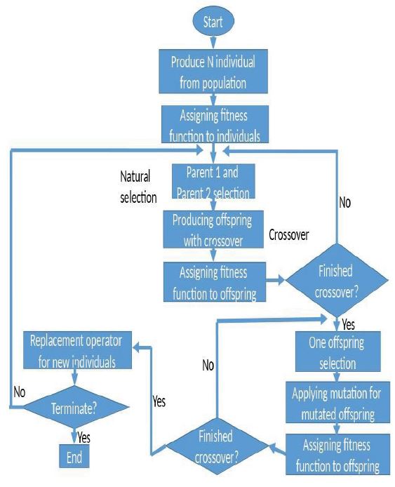
Figure 10: Genetic algorithm optimization scheduling algorithm flow chart. This shows the flow chart of the working principles of the genetic algorithm. The user or the client sends a request. The request is arranged in an orderly manner like the first come first serve. Then a fitness function is applied to see the best fit value for the chromosome which will be the parents. After this process, the three phases of the genetic algorithm (selection, crossover, and mutation) will take place. The best fit value from this process will be used to perform this process again until the satisfied value is gotten. Once the genetic algorithm is applied, it checks for the availability of the possible resource and is then executed using a virtual machine.

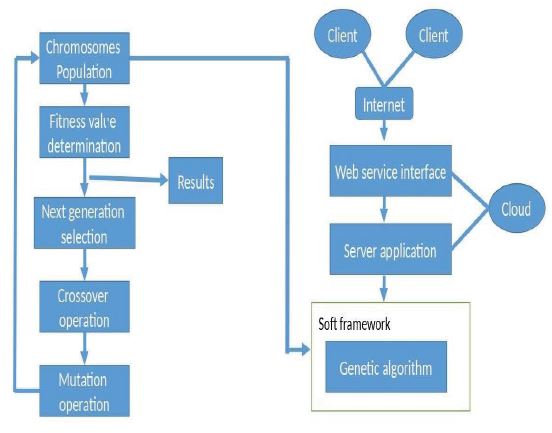
Figure 11: IoMT-cloud model of Genetic algorithm scheduling model. This illustrates the working principle of the proposed model on the IoT-cloud stage. The genetic operation (selection, crossover, and mutation) will take place in a soft framework situated in the cloud platform. Once the clients request the task, it is sent to the cloud stage where the checking for resources availability will take place and be executed using a virtual machine based on the soft framework.

• Fitness: Calculate the fitness estimation of these recently produced chromosomes known as offspring.

• Replacement: Update the population P by supplanting weak chromosome with better chromosomes from offspring.

• Repeat stages 3 to 7 until the halting condition is met. A halting condition might be the most extreme number of cycles or no adjustment in wellness estimation of chromosomes for successive emphases.

• Output the best chromosome as the last arrangement.

• End Procedure.

The calculation comprises three fundamental activities: introductory population, mutation, and finally crossover. These tasks are clarified beneath:

• Initial population age: GA deals with fixed piece string portrayal of individual arrangement. Thus, all the potential arrangements in the arrangement space are encoded into paired strings. From this, an underlying population of ten chromosomes is chosen.

• Crossover: The goal of this progression is to choose the majority of the occasions the best-fitted pair of people for crossover. This pool of chromosomes goes through an arbitrary single-point crossover, were relying on the crossover point, the bit lying on one side of the crossover site is traded with the opposite side. The fitness estimation of every individual chromosome is determined utilizing the fitness value. Subsequently, it creates another pair of people.

• Mutation: Depending upon the transformation esteem, the pieces of the chromosomes are flipped from 1 to 0 or 0 to 1. Presently a little worth (0.05) is gotten as mutation likelihood. The yield of this is another mating pool prepared for crossover.

The GA adjusts the heap in the IoMT-cloud by allocating errands to the virtual machines. It consistently appoints undertakings to a portion of the VMs. In any case, it isn’t successful in asset use which implies it neglects to use all the accessible virtual machines. Because of which a few machines stay inert while a few machines are over- burden. The proposed model monitors all the free virtual machines. The assets are not appropriately used. So this issue is handled by enhancement with the hereditary calculation. At the point when another errand shows up, first, it is watched that if a free machine is accessible and on the off chance that a machine is accessible, at that point task is allotted to that specific machine. In this manner, all the VMs are appropriately used and no VM stays inactive and no VM is overused. On the off chance that no free virtual machine is accessible, at that point, the undertaking is doled out to that machine whose current assignment will be finished in lesser time when contrasted with different machines. The proposed GA will give better yield as far as energy productivity, cost, total finish time (TFT), total waiting time (TWT), and all the VMs are distributed jobs.

Experimental process

The task scheduling framework in IoMT-cloud will go through three levels which are depicted beneath and the cycle of the hereditary calculation is portrayed in figure 12.

• The first level (Task): is a bunch of jobs that are sent by cloud clients, which are needed for execution.

• Second-level (scheduling): is answerable for planning jobs to appropriate assets to get the most elevated asset usage with the least makespan. The makespan is the general fulfillment time for all errands from the earliest starting point as far as possible.

• The third level (VMs): is a bunch of virtual machines which are utilized to execute the undertakings.

• A portion of the contemplations when scheduling jobs to VMs in the IoMT-cloud are.

• The number of jobs should be more than the quantity of VMs, which implies that each VM should execute more than one assignment.

• Each task is allocated to just a single VM asset.

• Lengths of undertakings fluctuating from little, medium, and enormous.

• Jobs are not interfered with once their executions start.

• VMs are autonomous regarding assets and control.

• The accessible VMs are of restrictive use and can’t be divided between various assignments. It implies that the VMs can’t consider different errands until the fruition of the current undertakings is in advancement.

In GA, the population statement is thoroughly examined to be the pre-processing, subsequently, its thickness isn’t considered for the survey. For the improvement utilizing GA in the wake of playing out the essential activity that implies when fitness computation, crossover activity, selection, and mutation activity are finished then the execution will end and the outcomes found. While programming into a paired string a period thickness of at most n1, for assessment of cost work 3 with maximum (c × k) for cost testing c of k quantity of chromosomes. The three activity of GA is incessant iteratively till the ending standards are met so the all-out time complexity is given by Equation 1. The election cycle mhas a period multifaceted nature of at generally m, for singlepoint hybrid, the time intricacy is all things considered m, where m is chromosome length and for change, at any spot, it is again

m. For better execution, the condition can be more successful for this situation.

G = O{n1 + (c × k) + (n2 + 1)(m + m + m)

Visualization

This is with the imaginative mind that the outcome is an outline that contains the assistance of using visual instruments, so the test results are depicted ordinarily. The significant inspiration driving portrayal is depicting

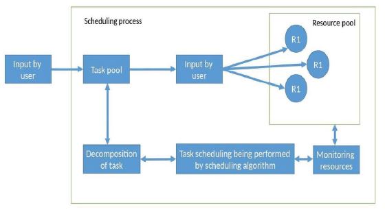
Figure 12: Genetic algorithm experimental process. This illustration shows how the experimental process is carried out. The user requests a task, the task will be arranged in an orderly manner. A decomposition process will occur while the genetic operation (selection, crossover, and mutation) takes place. The resources will be checked for availability so the appropriate tasks will be assigned to the appropriate resources based on a used algorithm. Once the genetic algorithm is applied, a monitoring process will take place to checks for task completion or the use of more resources.

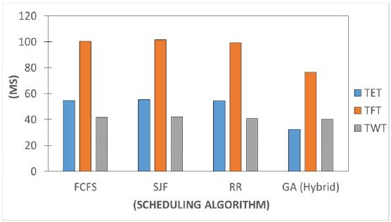
Figure 13: Depicting the TET, TFT, and TWT of all the scheduling models. This shows the correlation between each scheduling model against the TWT, TET, and the TFT. These are the used parameters to justify how efficient the model is. The timing parameters are highly considered when scheduling to attain a higher QoS. The result was analyzed using the same data to compare the performance of the algorithm. In RR, each work gets an equivalent measure of time, yet there are a few situations where normal waiting time can be an issue as shown in the results. After repeating the same test, our proposed hybrid model outperforms other models which are our baseline. The model has the least waiting time after optimization. This waiting time prevents users from waiting that long which avoids terminations. Moreover, the model produces the least execution time which makes the execution of tasks faster compared to other models. With this, we can determine the fairness within the task and which model to use in the time for scheduling.

the data and graphically conversing with it. The yield will be envisioned and discussed in the result portion. The example of data insight is depicted as stacking data into the application, data portrayal, and structure affirmation, showing the result, an example of portrayal is refined, at last examining the data.

Computational environment

The examinations done in this paper were executed using the eclipse IDE, which is an open-source condition that drives the utilization of SL strategies. Eclipse is a nopay and a standard programming condition that includes a solid set-up of instruments for information appraisal and genuine methodologies. Java is perhaps the most notable programming apparatus, and it offers various libraries that can manage data science endeavors, for instance, import datasets, data examination, data pre-taking care of, and specifically, working of models. Cloud is a bundle that sets forth various comprehensive limits concerning IoMT-cloud endeavors. It puts forth an attempt on different stages like Windows, macOS, or Linux, and with this current highlights can be joined. It is similarly the most characteristic and experienced language and it was used in this assessment. The experiment was surveyed on a pc with, intel focus i7 Processors: 2.3Ghz, GPU: EFORCE, RAM: 12GB, Disk: 1TB.

Results

To evaluate the feasibility of our method, we tried the planning cycle on different task scheduling algorithm models. Each model and highlight expect a fundamental
capacity to get the higher evaluation model. We have done a lot of various examinations with the most reassuring game plan of the scheduling calculations. The models have been attempted with different settings to achieve the most essential TWT, TET, TFT, accessibility, and calculation multifaceted nature. Also, numerous VMs were utilized and multiple tasks are utilized in this assessment. We have utilized three scheduling models FCFS, SJF, and RR to beat the expressed planning issue in IoMT-Cloud and subsequently enhancing it with an AI method known as GA. Each scheduling model demonstrates its proficiency while scheduling. At that point contrast the best-recognized scheduling model and appraisal metric communicated with other planning models. At the point when the best planning model is recognized, we see its productivity with the previously mentioned characteristics to best foresee these results. Each model utilized a comparative territory of instructive assortments. Eclipse and cloud sim was utilized which involves various libraries for this assignment. As follows the aftereffect of the models is explained in this part. In table 2 we portray a section of what the task length resembles.

Performance parameters and metrics

While contrasting the performance of the used task scheduling algorithms, these performance metrics below were utilized. Whereas, table 3 shows the tuning parameters used.

TWT (Total waiting time): The total waiting time is the absolute time spent by the process or job in the prepared state waiting to be executed. It is the time a task waits for execution when a few positions are contending in the scheduling system.

TET (Total execution time): The total execution time alludes to the time between the moment of submission of a job/process and the time of its culmination. Total execution time is the aggregate sum of time spent by the cycle from coming in the prepared state unexpectedly to its finishing. In this manner what amount of time it requires to execute a cycle is likewise a significant factor.

TFT (Total finish time): The total time at which a job or a process finishes its execution. It is the distance in time that lapses from the beginning of a job till it finishes.

Throughput: Throughput is the measure of work finished in a unit of time. The scheduling algorithm should hope to expand the number of tasks handled per time unit. Thus, throughput is the cycles executed to several tasks finished in a unit of time. It very well may be characterized as the number of cycles executed by the CPU in a given measure of time. Throughput is an approach to discover the proficiency of a CPU.

Status/Availability: This is a significant factor in concluding how to disperse and dispense the correct resources for a given VM. Knowing which assets are accessible at a given time. Asset accessibility assumes a principal part in the scheduling of tasks. The availability status is a success when the correct asset is being relegated to the VM.

Resource utilization: Resource utilization is another parameter that shows the maximization of the utilization of resources. This parameter is one of the main significance in task scheduling. Resources will be kept as busy. Whereas, service providers want to attain maxima gains by rendering a limited amount of resources. What is the amount of resources in the system that is busy, this helps in tracking the utilization of the system. Additionally, throughput and response time are significant, but another parameter for performance metrics for the system is the consumption of resources. Utilization of resources should be maximum in the scheduling system. The formula below shows how it is calculated, where n is the number of resources and i completions time for each resource.

Time is taken by resource i to finish all the task_{x n}

Average resource utilization = Makespan

Cost: This shows the economic cost which depicts the total amount that needs to be paid by the user to the service provider for the resource being utilized. This economic cost will be based on the quantity of time spent by the user on a particular resource. Table 4 below depicts the price factor in the unit. The formula below shows how it is calculated where T connotes the time the resource is being utilized and C connotes the economic cost of the resource per unit time.

cost = Σ {C × T}

i ∈ resources

The performance of the scheduling models

A large number of Virtual Machines runs inside a server

Task	Length (ms)
T1	70000
T2	100000
T3	5000
T4	10000
T5	90000
T6	15000
T7	25000
T8	200000
T9	150000
T10	60000

Table 2: Depiction of the task length.

Parameter	Value
Machine	0-14
Task	10-40
Algorithm	4
Data center	0-3

Table 3: Simulation Parameter.

Number of nodes	1	2	3	4	5	6	7	8
Price unit for each Operation	0.2	0.8	0.9	0.7	0.2	0.4	0.6	0.4

Table 4: Unit price per resource

Cloudlet ID	Status	Data center ID	VM ID	Execution Time	Start Time	Finish Time	Waiting Time
0	SUCCESS	2	0	1	0.1	1.1
1	SUCCESS	2	1	1.11	0.1	1.21
2	SUCCESS	2	2	1.11	0.1	1.21
3	SUCCESS	2	3	1.11	0.1	1.21
4	SUCCESS	2	4	1.11	0.1	1.21
5	SUCCESS	2	5	1.11	0.1	1.21
6	SUCCESS	2	6	1.11	0.1	1.21
7	SUCCESS	2	7	1.11	0.1	1.21
8	SUCCESS	2	8	1.11	0.1	1.21
9	SUCCESS	2	9	1.11	0.1	1.21
10	SUCCESS	2	10	1.11	0.1	1.21
11	SUCCESS	2	11	1.11	0.1	1.21
12	SUCCESS	2	12	1.11	0.1	1.21
13	SUCCESS	2	13	1.22	0.1	1.32
14	SUCCESS	2	14	1.22	0.1	1.32
15	SUCCESS	2	0	1.3	1.1	2.4	1
16	SUCCESS	2	1	1.31	1.21	2.51	1.11
17	SUCCESS	2	2	1.42	1.21	2.62	1.11
18	SUCCESS	2	3	1.42	1.21	2.62	1.11
19	SUCCESS	2	4	1.42	1.21	2.62	1.11
20	SUCCESS	2	5	1.42	1.21	2.62	1.11
21	SUCCESS	2	6	1.42	1.21	2.62	1.11
22	SUCCESS	2	7	1.42	1.21	2.62	1.11
23	SUCCESS	2	8	1.42	1.21	2.62	1.11
24	SUCCESS	2	9	1.42	1.21	2.62	1.11
25	SUCCESS	2	10	1.42	1.21	2.62	1.11
26	SUCCESS	2	11	1.42	1.21	2.62	1.11
27	SUCCESS	2	12	1.42	1.21	2.62	1.11
28	SUCCESS	2	13	1.42	1.32	2.73	1.22
29	SUCCESS	2	14	1.42	1.32	2.73	1.22
30	SUCCESS	2	0	1.6	2.4	4	2.3
31	SUCCESS	2	1	1.6	2.51	4.12	2.42
32	SUCCESS	2	2	1.61	2.62	4.23	2.53
33	SUCCESS	2	3	1.72	2.62	4.34	2.53
34	SUCCESS	2	4	1.72	2.62	4.34	2.53
35	SUCCESS	2	5	1.72	2.62	4.34	2.53
36	SUCCESS	2	6	1.72	2.62	4.34	2.53
37	SUCCESS	2	7	1.72	2.62	4.34	2.53

38	SUCCESS	2	8	1.72	2.62	4.34	2.53
39	SUCCESS	2	9	1.72	2.62	4.34	2.53

Table 5: Depiction of the FCFS scheduling algorithm results in seconds(s).

farm to use the assets in the most ideal way. Cloud providers have an enormous number of servers and other processing foundations. The scheduling will never really use the assets by dispensing explicit assignments to explicit assets. These scheduling calculations find the task with rent execution time and afterward appoint the asset to that task which creates the least execution time. It consequently improves the nature of administration and execution. If different assets give a similar measure of execution time, at that point asset is chosen on an irregular premise. The calculations work such that assignments are planned as they are shown up in the framework. The used scheduling models are FCFS, SJF, RR, and improvement utilizing the GA Algorithm. The execution of different scheduling calculations was done by utilizing clouds. To ensure model consistency, all models executed in this endeavor used a similar measure of assignment with different lengths. The results of the scheduling models will be found in the figures and tables underneath. The table contains the yield of the models on different test qualities has portrayed in the past sections. Moreover, as a result of the differentiation in the pre-handling process, the results were beneficial for each model. Also when we played out the models with default limits we similarly refined the GA with RR outperforms another model with regards to the QoS. Most of our displays with precision were applied with default limits from the beginning.

Utilizing the FCFS, a task that showed up first is served first. Tasks on the line are embedded into the tail of the line. Table 5 shows the aftereffects of the scheduling model per 40 assignments. Individually each cycle is taken from the head of the line. Though table 6 shows the total aftereffects of the scheduling model against our characteristics (TWT, TFT, TET). It shows it has little execution time, little completion time, and small waiting time. There is no prioritization at all and this makes each cycle to in the end finish before some other cycle is added. This calculation is clear and snappy. This shows the perception of the TWT, TFT, and TET of the tested FCFS. As setting switches possibly happens when a cycle is ended, hence no cycle line association is required and there is almost no scheduling overhead. This kind of calculation doesn’t function admirably with deferring touchy traffic as waiting time and postponement are generally on the higher side.

The SJF is pre-emptive in which it chooses the waiting cycle that has the least execution time. Table 7 shows the aftereffects of the planned errand per 40 assignments. While table 8 shows the total aftereffects of the scheduling model against our attributes (TWT, TFT, TET). It shows it has the most noteworthy execution time with a medium holding up time. One of the issues that SJF calculation is that it needs to become more acquainted with the following processor demand. The cycle is then apportioned to the processor that has the least blasted time. This shows the representation of the TWT, TFT, and TET of the tested SJF. It decreases the normal holding up time as it executes little cycles before the execution of huge ones. At the point when a framework is occupied with such countless more modest cycles, starvation will happen.

Traits	Throughput	Total Execution Time	Total Finish Time	Total waiting Time	Availability
Total	0.73	54.68	100.18	41.72	Success/40

Table 6: Depiction of the FCFS expected results traits in seconds (s).

Cloudlet ID	Status	Data center ID	VM ID	Execution Time	Start Time	Finish Time	Waiting Time
39	SUCCESS	2	0	1.02	0.1	1.12
38	SUCCESS	2	1	1.12	0.1	1.23
37	SUCCESS	2	2	1.12	0.1	1.23
35	SUCCESS	2	4	1.12	0.1	1.23
33	SUCCESS	2	6	1.12	0.1	1.23
31	SUCCESS	2	8	1.12	0.1	1.23
29	SUCCESS	2	10	1.12	0.1	1.23
27	SUCCESS	2	12	1.12	0.1	1.23
36	SUCCESS	2	3	1.12	0.1	1.23
34	SUCCESS	2	5	1.12	0.1	1.23
32	SUCCESS	2	7	1.12	0.1	1.23
30	SUCCESS	2	9	1.12	0.1	1.23
28	SUCCESS	2	11	1.12	0.1	1.23
25	SUCCESS	2	14	1.24	0.1	1.34
26	SUCCESS	2	13	1.24	0.1	1.34
24	SUCCESS	2	0	1.32	1.12	2.44	1.02
23	SUCCESS	2	1	1.33	1.23	2.55	1.12
22	SUCCESS	2	2	1.44	1.23	2.66	1.12
20	SUCCESS	2	4	1.44	1.23	2.66	1.12
18	SUCCESS	2	6	1.44	1.23	2.66	1.12
16	SUCCESS	2	8	1.44	1.23	2.66	1.12
14	SUCCESS	2	10	1.44	1.23	2.66	1.12
12	SUCCESS	2	12	1.44	1.23	2.66	1.12
21	SUCCESS	2	3	1.44	1.23	2.66	1.12
19	SUCCESS	2	5	1.44	1.23	2.66	1.12
17	SUCCESS	2	7	1.44	1.23	2.66	1.12
15	SUCCESS	2	9	1.44	1.23	2.66	1.12
13	SUCCESS	2	11	1.44	1.23	2.66	1.12
10	SUCCESS	2	14	1.44	1.34	2.77	1.24
11	SUCCESS	2	13	1.44	1.34	2.77	1.24
9	SUCCESS	2	0	1.62	2.44	4.06	2.34
8	SUCCESS	2	1	1.62	2.55	4.17	2.45
7	SUCCESS	2	2	1.63	2.66	4.29	2.56
5	SUCCESS	2	4	1.74	2.66	4.4	2.56
3	SUCCESS	2	6	1.74	2.66	4.4	2.56
1	SUCCESS	2	8	1.74	2.66	4.4	2.56
6	SUCCESS	2	3	1.74	2.66	4.4	2.56
4	SUCCESS	2	5	1.74	2.66	4.4	2.56
2	SUCCESS	2	7	1.74	2.66	4.4	2.56
0	SUCCESS	2	9	1.74	2.66	4.4	2.56

Table 7: Depiction of the SJF scheduling algorithm results in seconds (s).

Traits	Throughput	Total Execution Time	Total Finish Time	Total waiting Time	Availability
Total	0.72	55.36	101.67	42.21	Success/40

Table 8: Depiction of the SJF expected results traits in seconds (s).

Cloudlet ID	Status	Data center ID	VM ID	Execution Time	Start Time	Finish Time	Waiting Time
0	SUCCESS	2	0	1	0.1	1.1
1	SUCCESS	2	2	1	0.1	1.1
2	SUCCESS	2	4	1	0.1	1.1
4	SUCCESS	2	8	1	0.1	1.1
6	SUCCESS	2	12	1	0.1	1.1
3	SUCCESS	2	6	1	0.1	1.1
5	SUCCESS	2	10	1	0.1	1.1
7	SUCCESS	2	14	1	0.1	1.1
14	SUCCESS	3	13	1.13	0.1	1.23
8	SUCCESS	3	1	1.24	0.1	1.34
9	SUCCESS	3	3	1.24	0.1	1.34
10	SUCCESS	3	5	1.24	0.1	1.34
12	SUCCESS	3	9	1.24	0.1	1.34
11	SUCCESS	3	7	1.24	0.1	1.34
13	SUCCESS	3	11	1.24	0.1	1.34
22	SUCCESS	2	14	1.26	1.1	2.36	1
15	SUCCESS	2	0	1.37	1.1	2.47	1
16	SUCCESS	2	2	1.37	1.1	2.47	1
17	SUCCESS	2	4	1.37	1.1	2.47	1
19	SUCCESS	2	8	1.37	1.1	2.47	1
21	SUCCESS	2	12	1.37	1.1	2.47	1
18	SUCCESS	2	6	1.37	1.1	2.47	1
20	SUCCESS	3	10	1.37	1.1	2.47	1
29	SUCCESS	3	13	1.4	1.23	2.63	1.13
28	SUCCESS	3	11	1.4	1.34	2.75	1.24
23	SUCCESS	3	1	1.51	1.34	2.86	1.24
24	SUCCESS	3	3	1.51	1.34	2.86	1.24
25	SUCCESS	3	5	1.51	1.34	2.86	1.24
27	SUCCESS	3	9	1.51	1.34	2.86	1.24
26	SUCCESS	3	7	1.51	1.34	2.86	1.24
37	SUCCESS	2	14	1.53	2.36	3.89	2.26
36	SUCCESS	2	12	1.54	2.47	4.01	2.37
30	SUCCESS	2	0	1.65	2.47	4.12	2.37
31	SUCCESS	2	2	1.65	2.47	4.12	2.37
32	SUCCESS	2	4	1.65	2.47	4.12	2.37
34	SUCCESS	2	8	1.65	2.47	4.12	2.37
33	SUCCESS	2	6	1.65	2.47	4.12	2.37
35	SUCCESS	2	10	1.65	2.47	4.12	2.37
39	SUCCESS	3	3	1.73	2.86	4.59	2.75
38	SUCCESS	3	1	1.84	2.86	4.7	2.75

Table 9: Depiction of the RR scheduling algorithm results in seconds (s).

In the RR, measures are executed much the same as in FIFO, yet they are confined to processor time known as time-cut. Table 9 and table 10 shows the consequences of the scheduled task with per 40 undertaking. If the cycle isn’t finished before the termination on processor time, at that point the processor takes the following cycle in the holding upstate in the line. This shows the aggregate aftereffects of the planning model against our attributes (TWT, TFT, TET). It shows it has little execution time, the littlest completion time, and the least waiting time. The acquired or new cycle is then added to the back of the prepared rundown and afterward, new cycles are embedded in the tail of the line. If we apply quantum, at that point it will bring about helpless reaction time. If we apply a more limited quantum, at that point all things considered there will be lower CPU proficiency. As waiting time is high, there will be an extremely uncommon possibility that cutoff time will be met.

In this GA, need is allocated to each cycle, and cycles are executed based on need. Cycles with higher needs bring about the least waiting time and lesser deferral. If there is countless equivalent need, at that point it brings about enormous waiting time. Low organized cycles can see starvation. Table 11 shows the aftereffects of the planned errand per 40 tasks. It was productive with 143 counts and an efficient makespan. At the point when another task shows up, first, it is watched that if a free machine is accessible and on the off chance that a machine is accessible, at that point task is doled out to that specific machine. The Genetic Algorithm monitored mall the free virtual machines. While table 12 shows the total consequences of the scheduling model against our attributes (TWT, TFT, TET). On the off chance that no free virtual machine is accessible, at that point the task is allotted to that machine whose current assignment will be finished in lesser time when contrasted with different machines. Fitness assesses the nature of every posterity. In this manner, all the VMs are appropriately used and no VM stays inert and no VM is overused. The cycle is rehashed until adequate posterity is made. Three administrators to accomplish this are the crossover, selection, and mutation. The productivity of the GA relies on an appropriate blend of exploitation and investigation.

Experimental result discussion and comparison

Table 13 shows the correlation between all the models against the endorsed traits. Throughput with the proposed model is optimum. RR and GA Scheduling gives timesharing capacities. FCFS includes little execution time, little completion time, and small waiting time as short cycles wait for more extended spans. SJF is reasonable for practically all kinds of situations. With medium waiting time, for smaller processes, it isn’t suggested where delicate traffic is included. These results validate our approach towards getting an efficient model. Here we compare and contrast the

Traits	Throughput	Total ExecutionTime	Total Finish Time	Total waiting Time	Availability
Total	0.74	54.31	99.31	40.92	Success/40

Table 10: Depiction of the RR expected results traits in seconds (s).

Cloudlet ID	Status (success)	Data center	VM ID	Time of Execution	Time Start	Time Finish	Waiting Time
1	âœ“	2	11	0.75	0.1	0.85
0	âœ“	2	4	0.75	0.1	0.85
2	âœ“	2	7	0.75	0.1	0.85
5	âœ“	2	9	0.75	0.1	0.85
3	âœ“	2	1	0.75	0.1	0.85
6	âœ“	2	2	0.76	0.1	0.86
8	âœ“	2	6	0.76	0.1	0.86
11	âœ“	2	8	0.76	0.1	0.86
10	âœ“	2	10	0.76	0.1	0.86
4	âœ“	2	3	0.77	0.1	0.87
12	âœ“	2	13	0.77	0.1	0.87
16	âœ“	2	12	0.77	0.1	0.87
28	âœ“	2	5	0.77	0.1	0.87
39	âœ“	2	0	0.78	0.1	0.88
13	âœ“	2	11	0.81	0.85	1.66	0.75
7	âœ“	2	4	0.81	0.85	1.66	0.75
9	âœ“	2	3	0.81	0.87	1.68	0.77
17	âœ“	2	10	0.82	0.86	1.68	0.76
15	âœ“	2	2	0.82	0.86	1.68	0.76
24	âœ“	2	9	0.82	0.85	1.67	0.75
19	âœ“	2	1	0.83	0.85	1.68	0.75
27	âœ“	2	6	0.83	0.86	1.69	0.76
29	âœ“	2	8	0.83	0.86	1.69	0.76
36	âœ“	2	7	0.83	0.85	1.65	0.75
33	âœ“	2	12	0.83	0.87	1.70	0.77
38	âœ“	2	5	0.84	0.87	1.71	0.77
14	âœ“	2	11	0.81	1.66	2.47	1.56
22	âœ“	2	4	0.81	1.66	2.47	1.56
18	âœ“	2	10	0.81	1.68	2.49	1.58
26	âœ“	2	3	0.81	1.68	2.49	1.58
20	âœ“	2	2	0.82	1.68	2.50	1.58
34	âœ“	2	8	0.82	1.69	2.51	1.59
37	âœ“	2	6	0.82	1.69	2.51	1.59
21	âœ“	2	11	0.82	2.47	3.29	2.37
23	âœ“	2	10	0.82	2.49	3.31	2.39
30	âœ“	2	4	0.83	2.47	3.30	2.37
31	âœ“	2	2	0.83	2.50	3.33	2.40
25	âœ“	2	11	0.91	3.29	4.20	3.19
32	âœ“	2	4	1.01	3.30	4.31	3.20
35	âœ“	2	11	1.02	4.20	5.22	4.10

Table 11: Depiction of the optimized GA (hybrid) scheduling algorithm results in (ms).

Traits	Throughput	Total Execution Time	Total Finish Time	Total waiting Time	Availability
Total	1.23	32.47	76.6	40.16	Success/40

Table 12: Depiction of the optimized GA (hybrid) expected results traits in seconds (s).

Traits	FCFS	SJF	RR	GA
Throughput	0.73	0.72	0.74	1.23
Total Execution Time	54.68	55.36	54.31	32.47
Total Finish Time	100.18	101.67	99.31	76.6
Total waiting Time	41.72	42.21	40.92	40.16
Availability	Success/40	Success/40	Success/40	Success/40
Algorithm complexity	âœ“	âœ“	âœ“	âœ“

Table 13: Depiction of all the scheduling models against the traits in (ms).

each work gets an equivalent measure of time, yet there are a few situations where normal waiting time can be an issue as shown in the results. After repeating the same test, our proposed hybrid model outperforms other models which are our baseline. The model has the least waiting time after optimization. This waiting time prevents users from waiting that long which avoids terminations. Moreover, the model produces the least execution time which makes the execution of tasks faster compared to other models. The finish time of our model outperforms other models, in contrast with the fact that other models have a higher finishing time. With this, we can determine the fairness within the task and which model to use in the time for scheduling. While figure 14 shows the correlation against the throughput has we can see the best model with the best throughput is the hybrid model. The throughput is one of the best justifying parameters to show the performance of a process per unit time. After series of 40 task efforts were made to maximize the throughput. This is the highest number of tasks that can be completed per unit time, it outperforms another model. This result depicts how efficient our model is. Each task was split in their 10th to show the performance. During this course, we can see our model outperforms another model even during the split.

Figure 15 shows the correlation of resource utilization for the scheduling model. So, the idle waiting time is decreased in the proposed hybrid algorithm concerning other models. Furthermore, the proposed hybrid utilizes the resources that are free during the run time by choosing a new task. The resource utilized is compared under various cumulative counts of the makespan. Also, the resource utilization is enhanced respectively. However, when various other resources can be utilized then it becomes optimum. As the size of the resource, or the amount of task increase,N there is a normal rise in the average waiting time. The hybrid and RR have an increase in the resource utilized and then stay in a steady state. From the figure, we can also deduce the efficiency of other models in contrast to our model, the average resource utilized by other models remains almost similar, which means it is affected by the number of available resources. Therefore, we can conclude that the hybrid is the most efficient in contrast to the other sampled baseline models.

Figure 16 shows the economic cost factor. The result gotten shows the hybrid model per each task as a lesser cost factor. Cost is to notice the impact of the charged value rate over the used approach for data delivery. This impeding

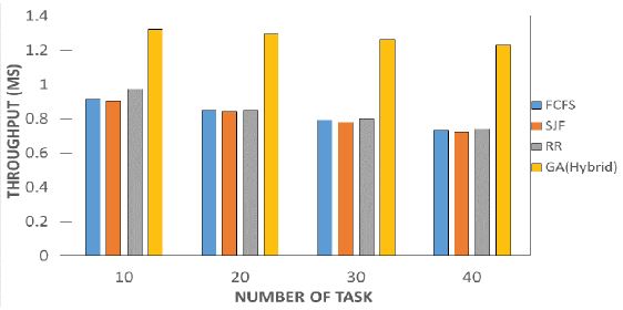
Figure 14: Depicting the throughput of all the scheduling models. This shows the correlation against the throughput has we can see the best model with the best throughput is the hybrid model. The throughput is one of the best justifying parameters to show the performance of a process per unit time. After series of 40 task efforts were made to maximize the throughput. This is the highest number of tasks that can be completed per unit time, it outperforms another model. This result depicts how efficient our model is. Each task was split into their 10th to show the performance. During this course, we can see our model outperforms another model even during the split.

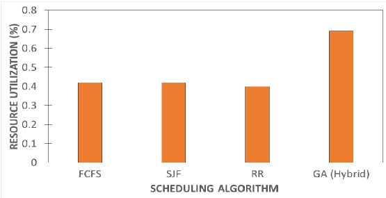
Figure 15: Depicting the resource utilization vs the scheduling models. This shows the correlation of resource utilization for the scheduling model. So, the idle waiting time will be decreased in the proposed hybrid algorithm concerning other models. Furthermore, the proposed hybrid utilizes the resources that are free during the run time by choosing a new task. The resource utilized is compared under various cumulative counts of the makespan. Also, the resource utilization is enhanced respectively. However, when various other resources are utilized then it becomes optimum. As the size of the resource, or the amount of task increase, there is a normal rise in the average waiting time. The hybrid and RR have an increase in the resource utilized and then stay in a steady state. From the figure, we can also deduce the efficiency of other models in contrast to our model, the average resource utilized by other models remains almost similar, which means it is affected by the number of available resources. Therefore, we can conclude that the hybrid is the most efficient in contrast to the other sampled baseline models.

advantage makes it more interesting for users without the fear of being overcharged. It is an evaluating factor for every hub in the IoT cloud pack. This was set as a level rate for every number of assets, where setting it to a moderately high worth would lessen the odds of the asset being chosen for a task. The baseline model shows a promising advantage where the percentage rate was on a similar value per task. Nevertheless, this won’t suit the user’s criteria as the utilization in the medical field will warrant a great amount of utilization time and this will increase the cost respectively. The result shows how to solve this problem with the proposed hybrid model to minimize the cost tremendously. We can conclude by stating the hybrid model surpasses expectations and as a minimum economical cost contrast to other baseline models.

Though in table 14 we portray the pros, cons, and the QoS of each model. Furthermore, how the experimented model will play a pivotal role in the medical field where resources are requested by the second. This shows that task scheduling is needed to attain maxima revenue when considering QoS and requests from the users. In this table, we can see our proposed hybrid outperformed other models with a substantial QoS. With this, medical data can be collected, analysis and monitoring. The Healthcare system can be digitalized to attain efficient connection of healthcare resources and services. Cloud users can answer incoming requests without the fear of a task being terminated or such. Thus, the trials show the hybrid beats other models and can be an efficient mode of scheduling for IoT-cloud in the medical field.

Conclusion

As we probably are aware, the IoMT-cloud is maybe unquestionably the most stimulating topic for scientists, public zone, and industry. This work presents the importance of the task scheduling calculations and kinds of static and dynamic task scheduling calculations in IoMTcloud climate. The improvement of distant correspondence and allocation of IoMT-cloud progressions grant issues that are being spouted by clients to be tackled remotely. The objective of the task scheduling test is to style a model nthat can close successful burdens while simultaneously sharing resources to get an efficient QoS. This assessment set forward depends on using present-day movements to improve practices on IoMT-cloud. This hypothesis targets building up a dynamic, sharp, and distinct framework for task scheduling in IoMT-cloud. We re-sanction the proposed estimation with different task scheduling models to show the adequacy of the proposed one after enhancement. This work likewise presents a relative report between the static and dynamic scheduling calculations in IoMTcloud-like the FCFS, SJF, RR, and advancement utilizing GA as far as TWT, TFT, TFT, and decency among tasks. This work will offer a possible manual for customers and specialists during IoMTcloud execution. We have thought about the aftereffect of the relative multitude of models and showed the outcomes. Experimentation was executed on CloudSim, which is utilized for displaying the various task scheduling calculations. From the charts and computations, it was demonstrated that the hybrid outshined other models with regards to execution time, cost resource utilization, and throughput calculation. It had a throughput of 1.23 and an execution rate of 32.47. GA with RR planning can be utilized in IoMT-cloud as the errand at the most punctual reaction time gets diminished viably. The diagrams and outcomes depict that the projected calculation is far superior to the next customary model when diverged from the instances of TWT, TET, and TFT. Subject to the measures while setting up this examination, future investigation is to be viewed like actualizing the calculationn for other advancement factors like lateness and stream time. Actualizing Hybrid streamlining calculation to get more

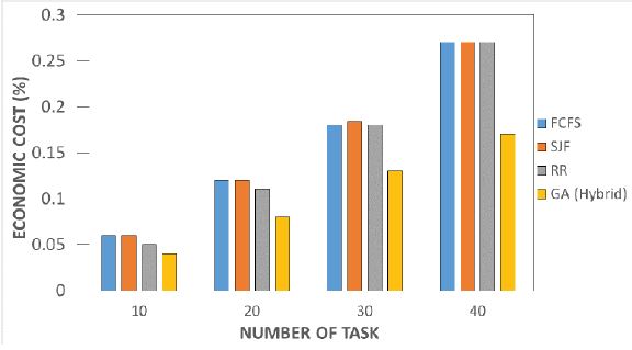
Figure 16: Depicting the economic cost vs the scheduling models. This shows the economic cost factor. The result gotten shows the hybrid model per task has a lesser cost factor. Cost is to notice the impact of the charged value rate over the used approach for data delivery. This impeding advantage makes it more interesting for users without the fear of being overcharged. It is an evaluating factor for every hub in the IoT cloud stage. The baseline model shows a promising advantage where the percentage rate was on a similar value per task. Nevertheless, this won’t suit the user's criteria as the utilization in the medical field will warrant a great amount of utilization time and this will increase the cost respectively. The result shows how to solve this problem with the proposed hybrid model to minimize the cost tremendously. We can conclude by stating the hybrid model surpasses expectations and has a minimum economical cost in contrast to other baseline models.

Scheduling model	Pros	Cons	QoS
FCFS	Implementation is straight forward.	No more scheduling criteria.	Little execution time, little finish time and little waiting time.
SJF	Scheduling was done to the task with minimum execution time.	Complexity in comprehending.	Highest execution time with medium waiting time.
RR	Complexity is less, with efficient balanced tasks.	It requires preemption.	Small execution time, smallest finish time and least waiting time.
GA	It is on the basis of several decision criteria, mutation, crossover and fitness function.	Complexity in coding and understanding.	Smallest execution time with the best throughput.

Table 14: Results pros, cons and QoS of the scheduling models.

improved outcomes. In future work, we can diminish the throughput time and Cost with the calculations to get more streamlined outcomes. Executing more AI strategies like PSO and Ant calculations. At long last, we will upgrade the work utilizing this characteristic as well and will bring the results as they will show up. It is accepted that this undertaking will help experts at whatever point considered. This is proposed to improve the adequacy of task scheduling for the IoMTcloud stage.

Declarations

Funding

The authors declare no funding.

Conflicts of Interest

The authors declare no conflict of interest.

Data Availability

The authors declare no data availability.

Supplementary Materials

The authors declare no supplementary material.

References

1. Armbrust M, Fox A, Griffith R, Joseph AD, Katz R, et al. (2010) A view of cloud computing. Communications of the ACM 53: 50-58.

2. Calheiros R N, Ranjan R, Beloglazov A, De Rose CAF, Rajkumar B (2011) CloudSim: a toolkit for modeling and simulation of cloud computing environments and evaluation of resource provisioning algorithms. Software: Practice and Experience 41: 23-50.

3. Zhu Zongbin, Du Zhongjun (2013) Improved GA-based task scheduling algorithm in cloud computing, Computer Engineering and Applications 49: 77-80.

4. Lijuan Z, Chunying W (2015) Cloud Computing Resource Schedulingin Mobile Internet Based on Particle Swarm Optimization Algorithm, Computer Science 42: 279-292.